
02 Jul Cassegrain Telescope with Fold Mirror
The following document will cover the analysis of a Cassegrain Telescope system. The polarization properties of the system will be measured with the Polaris-M software and the effects on imaging will be discussed. All plots and data have been generated with the Polaris-M software from Airy Optics, Inc.
Optical System
The optical system being analyzed is plotted below. The system consists of 5 optical surfaces:
- a stop (planar)
- the primary mirror (parabolic)
- the secondary mirror (hyperbolic)
- fold mirror (planar)
- detector/image plane (planar)
All optical surfaces are reflective and are coated with aluminum. An on-axis field will be traced with 0.55 μm rays.
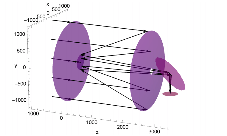
The units on the axes are [mm] and the telescope is approximately 3.5 meters long and 2 meters wide.
Surface Analysis
For any optical system, polarization aberrations can be introduced by reflection and refraction. The Fresnel coefficients at each surface will affect the light’s amplitude and phase differently for S-polarized and P-polarized light. This will introduce retardance and diattenuation. To manage the polarization, the optical designer needs baseline measurements of these retardance and diattenuation variations. Polaris-M comes with built-in functions to measure and plot the diattenuation and retardance variations at each surface. The polarization effects are plotted over the entire aperture for each surface to make what are called “Polarization Maps”. Polarization Maps can be generated for the angle of incidence (AOI), the retardance and the diattenuation.
Surface Polarization Maps
Nine Polarization maps for the Cassegrain Telescope are provided below. The first column (Blue) shows the AOI, the second column (Red) plots the diattenuation, and the third column (Purple) displays the retardance. The top row (Surface 2) plots the effects on the primary mirror, the second row (Surface 3) is the secondary mirror, and the bottom row (Surface 4) is the fold mirror. The magnitude of each plot is represented by the length of the line segment and the direction represents the plane of incidence for the AOI map (Blue), the diattenuation axis for the diattenuation map (Red), and the retardance axis or fast axis for the retardance map (Purple). Each map has a scale bar which is in radians for AOI (Blue) and Retardance (Purple). Diatteunation is unitless, with 0 implying no diattenuation, and 1 representing a perfect polarizer.
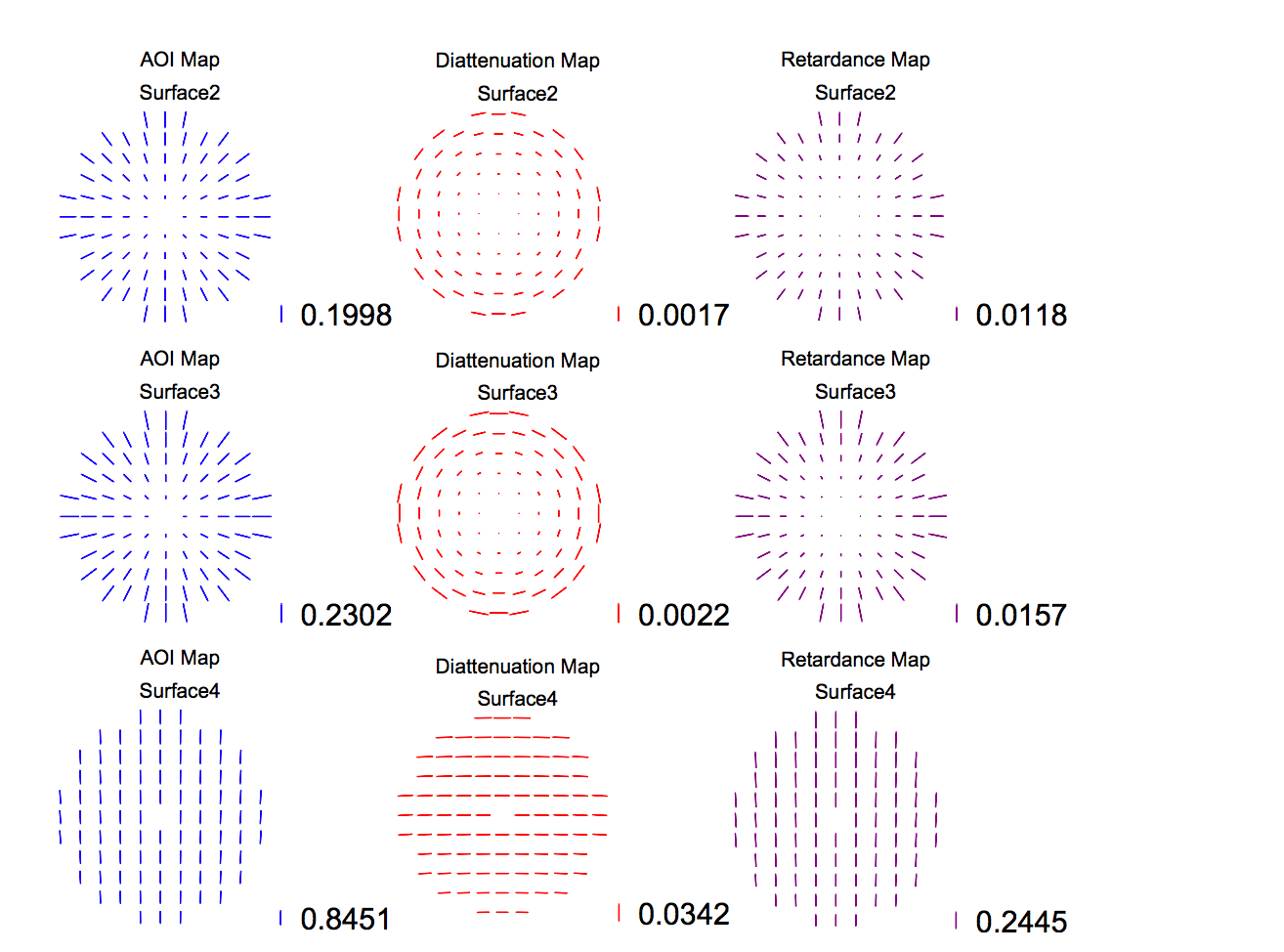
The AOI increased radially for both the primary and secondary mirror, so these surfaces act as radial retarders and polarizers. Similarly, the AOI is much greater across the fold mirror surface, so the fold mirror has more than 10 times the retardance and diattenuation.
Cumulative Polarization Maps
It is useful to plot the Polarization map for each surface so that the designer can see if a particular surface is the main contributing factor for the diattenuation and retardance; however, these effects will propagate and accumulate through the system. So, Polaris-M can be used to plot the cumulative Polarization Maps.
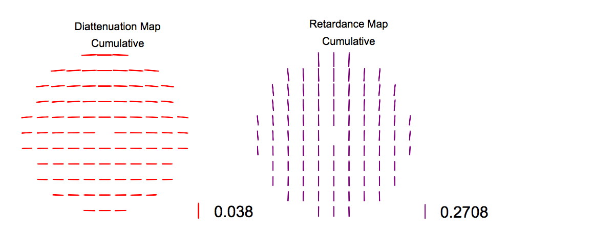
We see that the cumulative plots are dominated by the fold mirror. The primary and secondary mirrors contribute to the cumulative plot at the edges of the aperture, where the AOI is largest. These effects can be seen by the directions of the diattenuation and retardance axes at the edge of the aperture, which are rotated slightly in the radial direction.
Jones Pupil
As shown above, each surface affects the polarization, but how does this affect the imaging of the telescope? Polaris-M deals with this issue in a general manner by creating a Jones Pupil. A Jones Pupil is a matrix function that will give a 2 by 2 Jones Matrix to describe the polarization changes a particular ray will undergo after propagating through the optical system. This is a generalization of the wavefront aberration function to describe a polarized wavefront.
Polarization Basis
With a Jones Pupil, a 2-D representation of the electric field basis directions is used. A Jones matrix does this by making the assumption that the light is traveling in the Z-direction, and so the electric field will be in the X-Y plane. Since only the chief ray has this property in the telescope a basis function is needed to map the 3-D electric field vectors into a 2-D plane. Polaris-M can use both a Dipole basis and a Double Pole basis to perform the Global to Local transformation. For this telescope, a Double Pole basis was selected. The local e-field basis vectors (plotted in red and blue bellow) are displayed globally on the curved surface of the primary mirror.
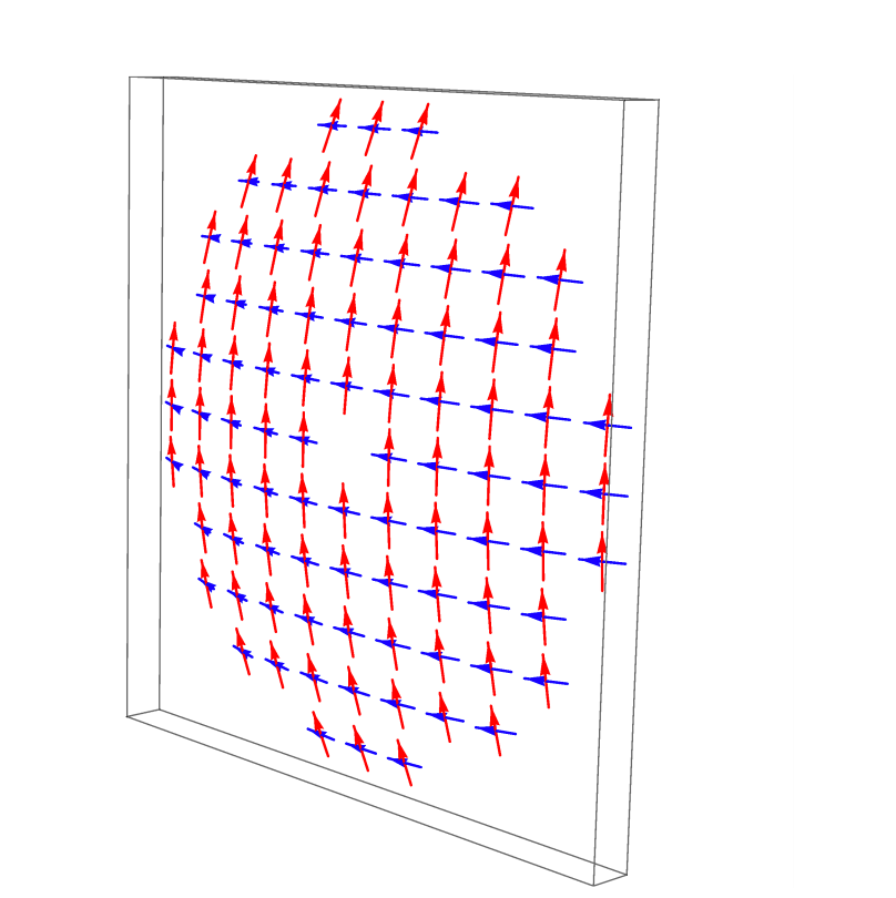
This basis will be used to create the Jones Pupil in the next section.
Jones Pupil Function
The Jones Pupil shows the polarization effects of the telescope system across the entire aperture, for any input polarization state. This function will change for each field of view similar to a wavefront aberration function. Additionally, the Jones Pupil is complex, so both the real and imaginary parts are plotted bellow (“Magnitude” → real part, “Phase” → imaginary part).
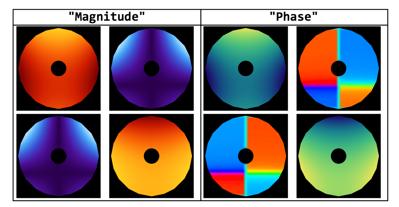
If this is a perfect system, we would get an Identity matrix. So the magnitude would be 1 along the diagonal and 0 along the off-diagonal for the entire aperture. Similarly, the imaginary parts would all be 0. Due to the diattenuation and retardance of the primary and secondary mirror, a cross pattern is visible in the Jones Pupil. The fold mirror has effectively shifted the cross down. These introduced aberrations will affect the point spread function and decrease the imaging quality of the system.
Polarized Point Spread Function (PSF)
In classical ray tracing, the Wavefront Aberration Function can be used to calculate the PSF; however, this does not include the polarization effects on imaging quality. With Polaris-M, the Jones Pupil Function can be used to generate a polarized PSF function, which will describe the PSF function for any polarization state.
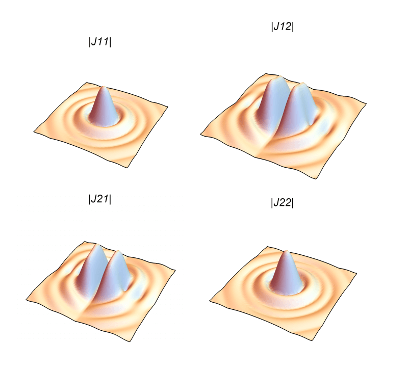
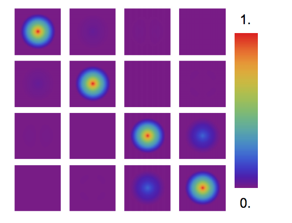
The J1,1 component describes the PSF function that would be measured if a horizontal polarizer was placed in front of the system and before the detector. The J2,2 component describes the PSF function that would be measured if a vertical polarizer was placed in front of the system and before the detector. The off-diagonal component J1,2, describes the PSF function that would be measured if a vertical polarizer was placed in front of the system and a horizontal polarizer was place before the detector. The off-diagonal component J2,1, describes the PSF function that would be measured if a horizontal polarizer was placed in front of the system and a vertical polarizer was place before the detector. Ideally (in an aberration free system), the Cassegrain telescope would produce a polarized PSF function with Airy Disk functions along the diagonal and 0 functions along the off diagonal.
PSF for Polarized Incident light
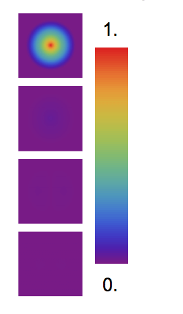
The polarized PSF can be used to get the point spread function for horizontally polarized light, by combing the J1,1 and J2,1 elements.
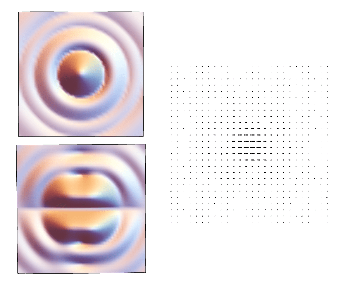
The plots on the left are the J1,1 and J2,1 elements, and the right plot show the combination where magnitude is represented by the length of the lines, and the polarization state is given by the direction of the lines. The PSF field is mostly horizontal; however, diattenuation from the primary, secondary and fold mirrors will rotate the polarization state slightly. Similarly, the retardance picked up from the mirrors can add ellipticity. This effect is more obvious with 45-degree incident light, due to the orientation of the fold mirror, which has a fast axis mostly in the Y-direction.

The plot on the left shows the 45-degree polarized PSF and the plot on the right is zoomed into the central lobe to show the ellipticity.
Mueller PSF/OTF
The Jones Pupil is great for analyzing polarized incident wavefront, but what if the incident light is incoherent/unpolarized? For this analysis Polaris-M can be used to generate Mueller PSF functions.
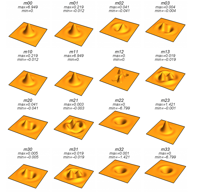
This function is equivalent to the polarized PSF generated from the Jones Pupil, but uses Mueller calculus to describe the Stokes parameters of the electric field.
Ideally, here we would have an Airy Disk function along the diagonal of the 4 by 4 Mueller PSF matrix.
Unpolarized OTF
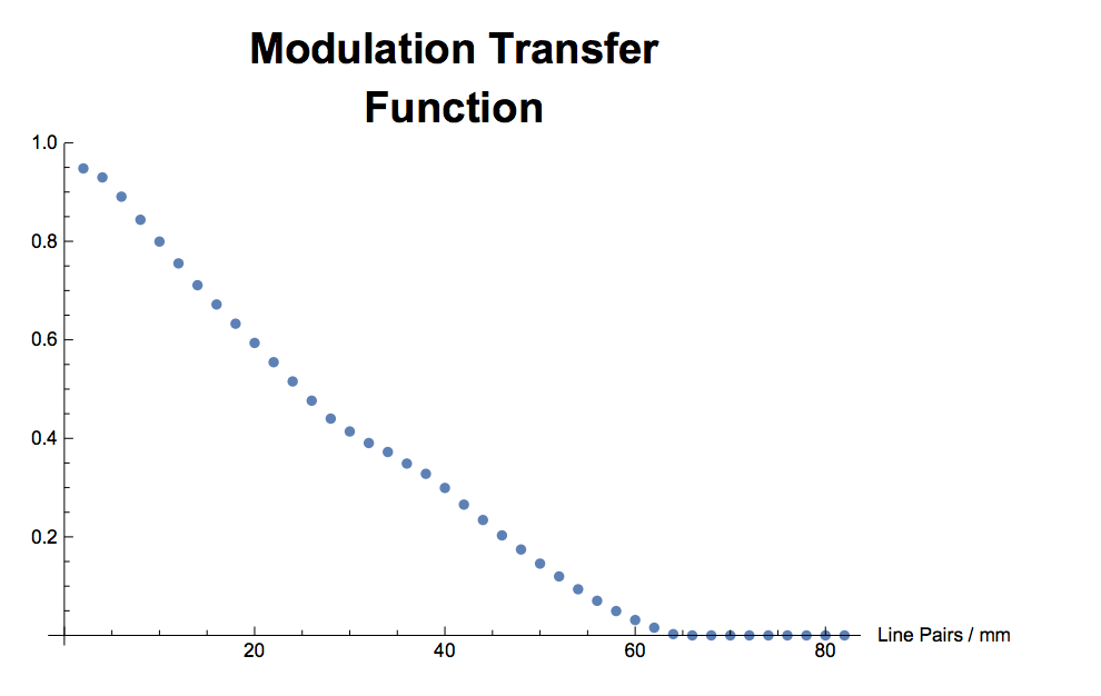
The PSF data can be used to calculate the Optical Transfer Function. Bellow the OTF is plotted in both the X and Y directions
The OTF for unpolarized light can be computed by combining the first column of the Mueller OTF.
The cross section can be plotted.
Summary
In conclusion, due the Fresnel coefficients, each element in the Cassegrain Telescope has polarization effects. These polarization effects vary spatially along the surface, and increase with the angle of incidence. Similarly, if the material at the optical interface changes, then the Fresnel coefficients will change, and so will the surface polarization effects. To analyze these effects on imaging, a Jones function is used. This function is a generalization of the Wavefront Aberration Function, and can be used to create the polarized PSF function. The polarized PSF function will give the PSF for any incident polarization state. If the incident light is unpolarized, a Mueller PSF function can be used.
No Comments